Blog

  • hacktoberfest-2023-participants

    Hacktoberfest-2023-Participants

    ⭐ Take part in Hacktoberfest 2023 by adding yourself to this website and by contributing your own web projects ⭐

    How to participate:

    Hello and welcome to Hacktoberfest 2023, I hope you are enjoying yourself!
    To take part in this repository, you can do multiple things:

    • Improve the design and features on the website itself.
    • Add yourself to the “Contributors” tab. Link your GitHub profile and tell us a few things about yourself, and add a project to ./contributor-projects that you would love to share with others.
    • Improve this documentation.

    (Additionally, if you could promote this to others so they can introduce themselves as well by leaving a star, that would mean a lot!)

    How to add yourself as a Contributor:

    It’s very simple. All you have to do is find the commented out HTML template in contributors.html, which contains everything already prepared for you. All you have to do is change the link to your profile picture (it can be external or you can add it to the repo), change the name, link to your GitHub, add your picture in the assets folder and give path of picture in the ‘src’ section of image part and of course change the description.
    Also, feel free to make your own custom CSS for your presentation, the more different styles, the better!

    HTML snippet:

    <div class="hacktoberfesr-contributor">
       <a href="GITHUB LINK HERE" target="_blank">
          <img class="mobile-img" src="ICON LINK HERE" height="150" width="150">
          <div class="card">
             <img class="desktop-img" src="ICON LINK HERE" height="400" width="400">
             <div class="card-info">
                <h1 class="orange-gradient">YOUR NAME</h1>
                <p class="flex-gap-small sub-info">Lorem Ipsum<span class="icon-circle"> o </span>Lorem Ipsum<span class="icon-circle"> o </span>Lorem Ipsum</p>
                <div class="using">
                   <h2>Software I use:</h2>
                   <div class="using-list">
                      <p>Lorem Ipsum</p>
                      <p>Lorem Ipsum</p>
                      <p>Lorem Ipsum</p>
                   </div>
                   <h2>Things I've developed with so far:</h2>
                   <div class="using-list">
                      <p>Lorem Ipsum</p>
                      <p>Lorem Ipsum</p>
                      <p>Lorem Ipsum</p>
                   </div>
                </div>
             </div>
          </div>
       </a>
    </div>

    Disclaimer for pull requests

    Although making a pull request by adding your profile is simple, the above mentioned snippet is what I prompt you to do after adding onto the website itself. Why do I say this? Because of the following rule of Hacktoberfest:

    Bad repositories will be excluded.
    
    PR/MRs should be useful to maintainers. Repos that encourage simplistic PR/MRs (like adding a name or profile to a list or arbitrarily curating content) will be excluded from Hacktoberfest. Remember: quantity is fun, quality is key.
    

    So even if your pull request does get accepted here, there is a chance that it won’t be added onto your valid record of completed Pull Requests. I will be adding Issues here for Hacktoberfest features, so there will be less confusion when it comes to accepted tasks.

    All the Issues will of course be here:

    Rules:

    There are not many rules. The only things you’d have to follow are:

    • Do not delete or alter any other people’s work or presentation,
    • Always make sure to sync this repo with your fork, because it can happen that someone might have commited changes right before you,
    • No auto redirects and keep all links target=”_blank”,
    • Pull requests shouldn’t be considered as “spammy”,
    • Be kind and show respect to everyone!

    After everything mentioned is done, I will check pull requests, add it to this repo and add the hacktoberfest-accepted label.

    That’s it!

    That’s gonna do it for this explaination! Have fun and best of luck on your Hacktoberfest journey!

    Visit original content creator repository
    https://github.com/Jan-Fcloud/hacktoberfest-2023-participants
  • DesignPattern

    DesignPattern

    Jungle设计模式系列

    How to compile

    Windows

    mkdir build
    cd build
    cmake -G "MinGW Makefiles" ../
    make
    

    Linux

    mkdir build
    cd build
    cmake ../
    make
    

    感谢

    感谢@ichdream, @sterben-01对本项目的贡献,也欢迎和支持更多coder提出修改和指正

    订正

    • 2021/10/28:GB2312 –> UTF-8
    • 2021/09/07:merge @ichdream pull request,采用智能指针管理堆对象,引入makefile管理工程,修改文件编码格式
    • 2021/04/04:为虚基类添加虚析构函数,避免内存泄露
    • 2020/11/29:解决内存泄露问题
    • 2023/09/24:添加CMake编译工程管理
    • 2024/04/17: update markdown note.

    目录

    代码资源:https://github.com/FengJungle/DesignPattern

    01.设计模式——设计模式概述

    02.设计模式(二)——UML类图介绍

    03.设计模式(三)——面向对象设计原则

    04.设计模式(四)——简单工厂模式

    05.设计模式(五)——工厂方法模式

    06.设计模式(六)——抽象工厂模式

    07.设计模式(七)——建造者模式

    08.设计模式(八)——原型模式

    09.设计模式(九)——单例模式

    10.设计模式(十)——适配器模式

    11.设计模式(十一)——桥接模式

    12.设计模式(十二)——组合模式

    13.设计模式(十三)——装饰模式

    14.设计模式(十四)——外观模式

    15.设计模式(十五)——享元模式

    16.设计模式(十六)——代理模式

    17.设计模式(十七)——职责链模式

    18.设计模式(十八)——命令模式

    19.设计模式(十九)——解释器模式

    20.设计模式(二十)——迭代器模式

    21.设计模式(二十一)——中介者模式

    22.设计模式(二十二)——备忘录模式

    23.设计模式(二十三)——观察者模式

    24.设计模式(二十四)——状态模式

    25.设计模式(二十五)——策略模式

    26.设计模式(二十六)——模板方法模式

    其他

    27.设计模式那么多!面试官会怎么问?

    博客地址:https://zhuanlan.zhihu.com/p/415609134

    28.划重点:面试中单例模式的考点!(C++版本)

    博客地址:https://zhuanlan.zhihu.com/p/692662459

    29.new也可以创建对象,为什么需要工厂模式?

    博客地址:https://zhuanlan.zhihu.com/p/611234726

    30.Qt中的设计模式

    博客地址:https://blog.csdn.net/sinat_21107433/article/details/120936720

    31.PImpl模式

    博客地址:https://zhuanlan.zhihu.com/p/692661653

    32.啊,如何遵循“低耦合”设计原则?

    博客地址:https://zhuanlan.zhihu.com/p/473171832

    Visit original content creator repository
    https://github.com/FengJungle/DesignPattern

  • php-mvc-pdo

    Estudando PHP em MVC com PDO

    Construindo uma aplicação PHP, com a finalidade de estudo, com rotas controles e classes de modelos utilizando de PDO e estrutura MVC para o projeto.

    Há inúmeros frameworks fantásticos para PHP, no mercado. Porém, com a finalidade de estudo, acho muito interesante a ideia de se construir do 0 toda a aplicação.

    Claro que a segurança e integridade que grandes frameworks chegam a ter, não conseguimos alcançar com este experimento. Mas nosso conhecimento chega a ter um BUM a mais.

    Começando com as Rotas

    Criei um arquivo simples no diretório App, que recebe as Rotas de uma forma simples.

    GET, POST, PUT, DELETE:

    use App\Http\Route;
    
    Route::get('/', "HomeController@index");
    
    Route::post('/users/create', "UserController@create");
    
    Route::put('/users/[0-9]+/update/', "UsersController@update");
    
    Route::get('/users/[0-9]+/delete/', "UsersController@delete");

    Desta forma, de maneira bem simplicada se declara Rotas.

    Bind values:

    Se preciso guardar informações, há uma classe pronta para isto.

    use App\Bind;
    
    Bind::add($key, $value);

    Passando uma chave e um valor, para ser coletado quando precissar chamando o metodo get da classe.

    Para buscar somente passando o $key.

    $appName = Bind::get('app-name');

    Controllers

    Controllers quando precisar de parâmetros deve se usar array.

    namespace App\Controllers;
    
    class MeuController extends Controller {
        public function index(array $params) {
            echo $params;
        }
    }

    Request

    As requests estão bem simples no momento, passando somente por filtro padrão do php.

    namespace App\Controllers;
    
    class MeuController extends Controller {
        public function index(Request $request) {
            echo $request->all();
        }
    }
    namespace App\Controllers;
    
    class MeuController extends Controller {
        public function index(Request $request) {
            echo $request->get("name");
        }
    }

    Por padrão está retornando objetos no all e o get

    namespace App\Controllers;
    
    class MeuController extends Controller {
        public function index(Request $request) {
            echo $request->_(); // Aqui retorna sem nada de filtro e como array
        }
    }

    Validate

    A classe validation no momento só faz validação padrão do PHP, e tem que receber um array para filtrar os dados.

    namespace App\Controllers;
    
    use App\Http\Validation;
    
    class MeuController extends Controller {
        public function index(Request $request) {
            $value = $request->_();
    
            $value = Validation::validate($value);
        }
    }

    Middlewares

    Adcionando middlewares no projeto.

    Primeiro passo é adicionar como 3° parâmetro na rota, um array com a string que deseja usar para o middleware. O mesmo que vamos cadastrar no mapeamento de classes.

    use App\Http\Route;
    
    Route::get('/', "HomeController@index", ["middleware"]);
    
    Route::post('/users/create', "UserController@create");
    
    Route::put('/users/[0-9]+/update/', "UsersController@update");
    
    Route::get('/users/[0-9]+/delete/', "UsersController@delete");
    Visit original content creator repository https://github.com/jacksonsr451/php-mvc-pdo
  • belajar-istio

    Belajar Istio Service Mesh

    About

    This is a repository of my learning results about Istio Service Mesh.

    Prerequisites

    • Kubernetes Cluster
    • Helm
    • Helmfile

    Components

    Here are the components that are included in this repository:

    • Istio
    • mTLS
    • Ingress Gateway
    • Authentication with JWKS
    • Kiali Dashboard
    • Prometheus
    • Grafana
    • Jaeger Tracing

    Installation

    1. Clone the repo

      git clone https://github.com/rizalord/belajar-istio.git
    2. Move to chart directory

      cd belajar-istio/chart
    3. Install all chart dependencies

      helmfile apply --concurrency=1
    4. Set label to default namespace

      kubectl label namespace default  istio-injection=enabled --overwrite
    5. Install main chart

      helm install belajar-istio .

    Access Kiali Dashboard

    1. Get the status of kiali installation

      kubectl get kiali kiali -n istio-system -o jsonpath='{.status}'
    2. Wait until property progress.message is equal to “7. Finished all resource creation”.

    3. Port forward kiali service

      kubectl port-forward svc/kiali 20001:20001 -n istio-system
    4. Open browser and go to http://localhost:20001

    API Documentation

    • Coming soon

    What I’ve Learned

    While working on this project, I have learned a few things and here are some of my highlights:

    1. Istio provide mTLS feature that can be used to secure communication between services. This feature can be enabled by default with no configuration needed.

    2. Istio will automatically inject a sidecar container to every pod that has the label istio-injection=enabled. This sidecar container will be used to intercept the traffic and do the mTLS.

    3. When we want to add a JWT Authentication, we can’t use the symmetric approach. We have to use the asymmetric approach which is using JWKS. With this approach, all service that need authentication will have to fetch the JWKS from the JWKS URL. Instead of having to fetch JWKS for every incoming request, it’s better to use a cache to store JWKS data.

    4. Istio provide a dashboard called Kiali that can be used to visualize the traffic between services. To install Kiali, we must install Prometheus first. After that we need to install Grafana and Jaeger (optional). After all of the components are installed, we can install Kiali.

    5. Workload in Istio means a pod, not a deployment.

    6. Gateway basically is an Ingress. So when we deploy it (eg. GKE), it will create a Load Balancer. Then when we want from outside (public) to access our cluster, we need to create a DNS record that points to the Load Balancer IP.

    Visit original content creator repository
    https://github.com/rizalord/belajar-istio

  • mec2

    mec2

    --{{0}}--
    

    This document defines some basic macros for applying the
    mec2 2D physics simulation in
    LiaScript.

    Try it on LiaScript:

    https://liascript.github.io/course/?https://raw.githubusercontent.com/LiaTemplates/mec2/main/README.md

    See the project on Github:

    https://github.com/liaTemplates/mec2

    --{{1}}--
    

    There are three ways to use this template. The easiest way is to use the
    import statement and the url of the raw text-file of the master branch or any
    other branch or version. But you can also copy the required functionionality
    directly into the header of your Markdown document, see therefor the
    last slide. And of course, you could also clone this project
    and change it, as you wish.

    {{1}}
    
    1. Load the macros via

      import: https://raw.githubusercontent.com/LiaTemplates/mec2/main/README.md

    2. Copy the definitions into your Project

    3. Clone this repository on GitHub

    @mec2

    --{{0}}--
    

    Simply add @mec2 directly to the head of your Markdown code-snippet to execute
    it directly within LiaScript.

    {
      "id":"chaos-pendulums",
      "gravity":true,
      "nodes": [
        { "id":"A0","x":200,"y":400,"base":true },
        { "id":"A1","x":280,"y":480,"m":2 },
        { "id":"B1","x":279,"y":481,"m":2 },
        { "id":"C1","x":278,"y":482,"m":2 },
        { "id":"D1","x":277,"y":483,"m":2 },
        { "id":"A2","x":360,"y":560,"m":3 },
        { "id":"B2","x":359,"y":561,"m":3 },
        { "id":"C2","x":358,"y":562,"m":3 },
        { "id":"D2","x":357,"y":563,"m":3 },
        { "id":"A3","x":440,"y":640,"m":4.7 },
        { "id":"B3","x":439,"y":641,"m":4.7 },
        { "id":"C3","x":438,"y":642,"m":4.7 },
        { "id":"D3","x":437,"y":643,"m":4.7 }
      ],
      "constraints": [
        { "id":"a1","p1":"A0","p2":"A1","len":{ "type":"const" } },
        { "id":"a2","p1":"A1","p2":"A2","len":{ "type":"const" } },
        { "id":"a3","p1":"A2","p2":"A3","len":{ "type":"const" } },
        { "id":"b1","p1":"A0","p2":"B1","len":{ "type":"const" } },
        { "id":"b2","p1":"B1","p2":"B2","len":{ "type":"const" } },
        { "id":"b3","p1":"B2","p2":"B3","len":{ "type":"const" } },
        { "id":"c1","p1":"A0","p2":"C1","len":{ "type":"const" } },
        { "id":"c2","p1":"C1","p2":"C2","len":{ "type":"const" } },
        { "id":"c3","p1":"C2","p2":"C3","len":{ "type":"const" } },
        { "id":"d1","p1":"A0","p2":"D1","len":{ "type":"const" } },
        { "id":"d2","p1":"D1","p2":"D2","len":{ "type":"const" } },
        { "id":"d3","p1":"D2","p2":"D3","len":{ "type":"const" } }
      ],
      "views": [
        { "show":"pos","of":"A3","as":"trace","id":"view1","stroke":"rgba(255,0,0,.5)" },
        { "show":"pos","of":"B3","as":"trace","id":"view2","stroke":"rgba(0,255,0,.5)" },
        { "show":"pos","of":"C3","as":"trace","id":"view3","stroke":"rgba(255,255,0,.5)" },
        { "show":"pos","of":"D3","as":"trace","id":"view4","stroke":"rgba(255,0,255,.5)" }
      ]
    }

    @mec2.eval

    --{{0}}--
    

    Attach @mec2.eval to the end of your Markdown code-snippet to create an
    editable and executeable simulation.

    {
      "id":"chaos-pendulums",
      "gravity":true,
      "nodes": [
        { "id":"A0","x":200,"y":400,"base":true },
        { "id":"A1","x":280,"y":480,"m":2 },
        { "id":"B1","x":279,"y":481,"m":2 },
        { "id":"C1","x":278,"y":482,"m":2 },
        { "id":"D1","x":277,"y":483,"m":2 },
        { "id":"A2","x":360,"y":560,"m":3 },
        { "id":"B2","x":359,"y":561,"m":3 },
        { "id":"C2","x":358,"y":562,"m":3 },
        { "id":"D2","x":357,"y":563,"m":3 },
        { "id":"A3","x":440,"y":640,"m":4.7 },
        { "id":"B3","x":439,"y":641,"m":4.7 },
        { "id":"C3","x":438,"y":642,"m":4.7 },
        { "id":"D3","x":437,"y":643,"m":4.7 }
      ],
      "constraints": [
        { "id":"a1","p1":"A0","p2":"A1","len":{ "type":"const" } },
        { "id":"a2","p1":"A1","p2":"A2","len":{ "type":"const" } },
        { "id":"a3","p1":"A2","p2":"A3","len":{ "type":"const" } },
        { "id":"b1","p1":"A0","p2":"B1","len":{ "type":"const" } },
        { "id":"b2","p1":"B1","p2":"B2","len":{ "type":"const" } },
        { "id":"b3","p1":"B2","p2":"B3","len":{ "type":"const" } },
        { "id":"c1","p1":"A0","p2":"C1","len":{ "type":"const" } },
        { "id":"c2","p1":"C1","p2":"C2","len":{ "type":"const" } },
        { "id":"c3","p1":"C2","p2":"C3","len":{ "type":"const" } },
        { "id":"d1","p1":"A0","p2":"D1","len":{ "type":"const" } },
        { "id":"d2","p1":"D1","p2":"D2","len":{ "type":"const" } },
        { "id":"d3","p1":"D2","p2":"D3","len":{ "type":"const" } }
      ],
      "views": [
        { "show":"pos","of":"A3","as":"trace","id":"view1","stroke":"rgba(255,0,0,.5)" },
        { "show":"pos","of":"B3","as":"trace","id":"view2","stroke":"rgba(0,255,0,.5)" },
        { "show":"pos","of":"C3","as":"trace","id":"view3","stroke":"rgba(255,255,0,.5)" },
        { "show":"pos","of":"D3","as":"trace","id":"view4","stroke":"rgba(255,0,255,.5)" }
      ]
    }

    @mec2.eval

    Implementation

    script: https://jauhl.github.io/mecEdit/scripts/g2.js
            https://jauhl.github.io/mecEdit/scripts/mec2.min.js
            https://jauhl.github.io/mecEdit/scripts/mecelement/canvasInteractor.js
            https://jauhl.github.io/mecEdit/scripts/mecelement/g2.selector.js
            https://jauhl.github.io/mecEdit/scripts/mecelement/mec.htmlelement.js
    
    
    @mec2
    <lia-keep>
    <MEC-2 width=800 height=600 grid cartesian darkmode x0=385 y0=139 >
    @0
    </MEC-2>
    </lia-keep>
    @end
    
    @mec2.eval: @mec2.eval_(@uid)
    
    @mec2.eval_
    <script>
    let json=`@input`
    
    document.getElementById("@0").innerHTML = "<MEC-2 id='test' width=1530 height=680 grid cartesian darkmode x0=385 y0=139 >" + json + "</MEC-2>"
    
    "LIA: stop"
    </script>
    
    <div id="@0"></div>
    
    @end

    Visit original content creator repository
    https://github.com/LiaTemplates/mec2

  • Molecular-Binding-Algorithm-by-Surface-Mapping-MBASM

    Molecular Adsorption by Surface Mapping Algorithm

    The present algorithm generates sets of atomic structures of adsorbed molecules, considering ridge structures and atoms as spheres of VDW radius (or a fraction of it).

    Input structure 1 Input structure 2 Result Structures
    A.xyz + B.xyz >>> AB_1.xyz AB_1_surf_km.xyz
    AB_n.xyz AB_n_surf_km.xyz

    Methodology

    Our methods mimic the ideia that two melecules could interact based on different chemical environments on the surface of the molecules. First, it get a representative sets of chemical environments of each one of the molecules. Second, we find structures combining the molecules through each possible pair of chemical environments in the molecules. Finally, this poll of structures is sampled to find a representative set of thepossible ways of interaction.

    Surface Mapping

    The objective of this step is to get a set of K points on the surface of each molecule, these points must represent the diversity of different chemical environments around the molecule:

    • Read the mol and associate VDW radii for each atom: There are VDW radii for some atoms (and their reference), but one can add VDW raddi manually, search for “add_your_vdw_radii_here” in the adsorption.py file.

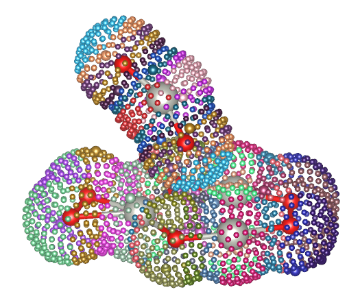
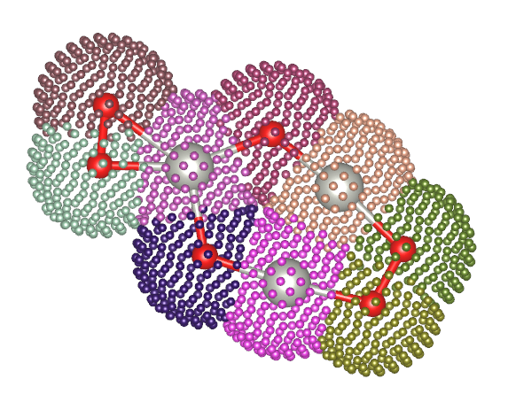
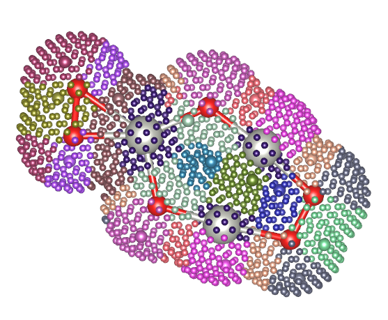
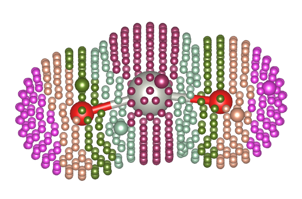
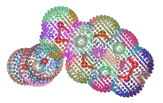
    • Both molecule surfaces are mapped with dots: The surface of a molecule is an outside surface built with the union of ridge spheres of VDW radii around each atom. The files mol_a_surf.xyz and mol_b_surf.xyz present this data [a]. Points in these spheres (SO2) are obtained with the algorithm describedby Deserno (see the article “How to generate equidistributed points on the surface of a sphere”, https://www.cmu.edu/biolphys/deserno/pdf/sphere_equi.pdf).

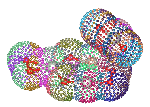
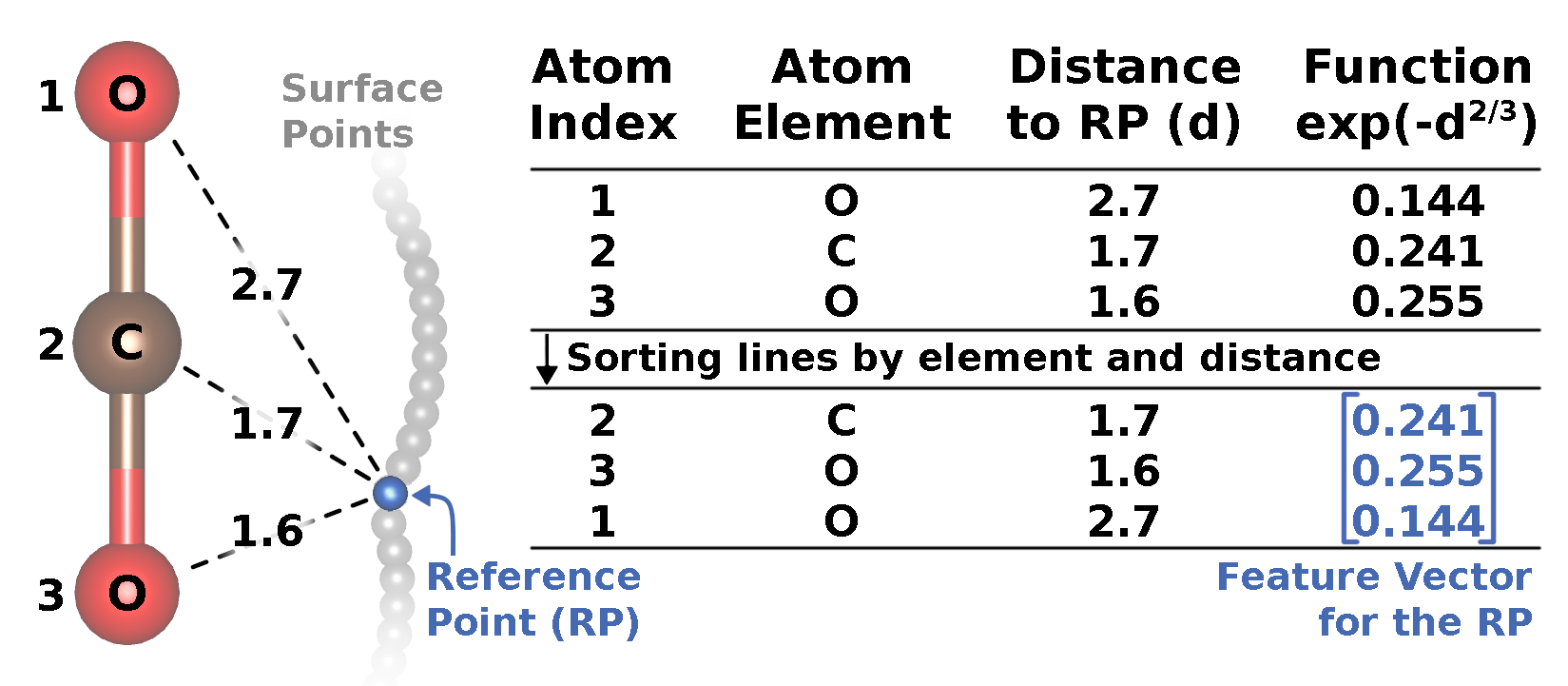
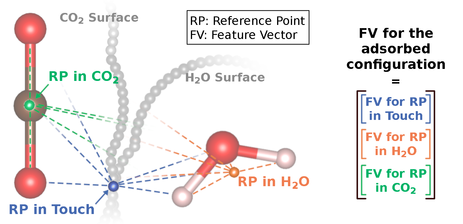
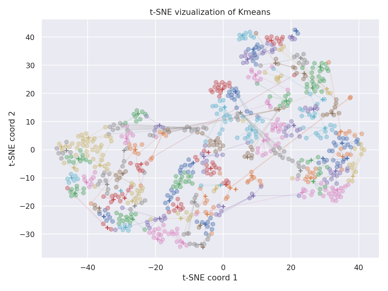
    • Featurize, clusterize and find representative dots among the surface dots. For each point of the surface, a feature vector is calculated as presented in the image below. The feature vector present an entry per atom. The order of the entries is sorted by chemical element and distances from the reference point in the surface to the atom. Then, based on a K-means clustering employed with these features data, the surface dots are grouped. The groups represent regions with similar chemical environment. The surface point with the features nearest to the mean feature values of each cluster is selected as a representative point in the molecular surface. The files mol_a_km.xyz and mol_b_km.xyz present this data [a].

    The files written during the surface mapping:
    Input structures (*.xyz)
    Surface dots (*_surf.xyz)
    Surface dots clustering (*_km.xyz)
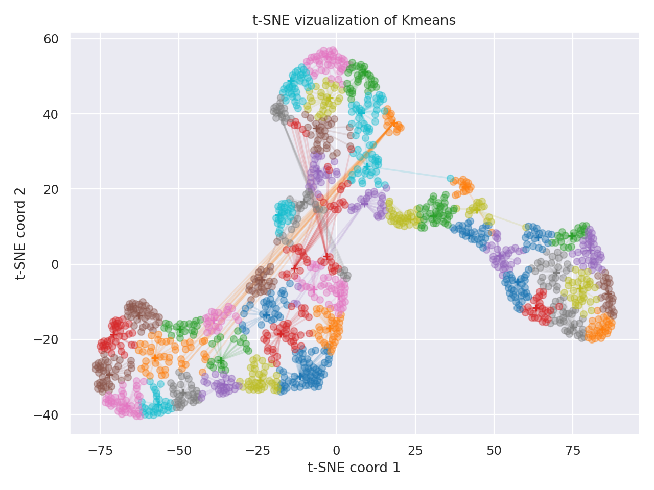
    Clustering in t-SNE reduced features

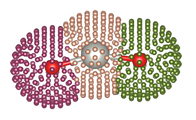
    The *_surf.xyz files present the surface dots with a color for the points associated with each atom. The *_km.xyz files present the surface dots with a color for the points associated with each cluster of surface dots. Similar colors of different figure have no relation with each other.

    The structure with the surface dots can be seen in the VESTA code. To correct read their data, you must replace the VESTA configuration file elements.ini with the elements.ini file added in the present project. These files present the types of atoms, colors, and other properties to automatically add colors to the representation.

    Adsorption

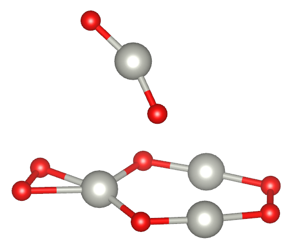
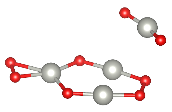
    The objective of this step is to obtain a pull with many and diverse adsorbed structures. Adsorption is performed by combining both molecules by each pair of the representative point of its surfaces. Moreover, for each pair of representative points, many rotations are performed to guarantee good matches between the molecules. These rotations are performed with a grid of rotations of SO3, obtained with a method called Successive Orthogonal Images on SOn. The method was first presented by Mitchell (DOI:10.1137/030601879), but for the present implementation I followed the paper by Yershova (DOI:10.1177/0278364909352700). Note that, the number of adsorbed molecules configurations to analyze is deterministic and is the product of the number of surface clusters for each molecule and the number of rotations in SO3.

    A configurations is added to a pull when:

    • The molecules did not overlap in the adsorption, which is considered to have happened when a pair of atoms of different molecules were distant by less than the sum of their VDW radii multiplied by the parameter ovlp_threshold. The parameter in general is above 0.90 and is important to guarantee that a adsorbed configurations generated are plausible.

    • The present adsorbed configuration should be different to any other adsorbed configuration in the pull of structures, which is verify with a simple filtering. The filtering is based on the euclidian distance between a feature vector for the present adsorbed configuration and all others feature vectors for the structures in the pull were larger than sim_threshold parameter, the present structure will be included in the pull. For each adsorbed configuration a feature vector is calculated as presented in the figure below.

      Note that this feature vector is equivalant to the concatenation of three feature vectors similar as the ones calated for suface points but only one reference point is on the surface. Two reference points are in the geometrical center of the molecules seapartedly. The last reference point is the position were the two representative surface dots are combined to create the present adsorbed configuration. The parameter must be setted acording to each pair of structures and is important to avoid overrpresenting some regions of the space of adsorption configurations.

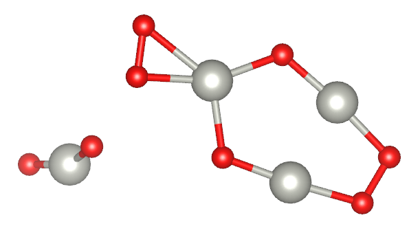
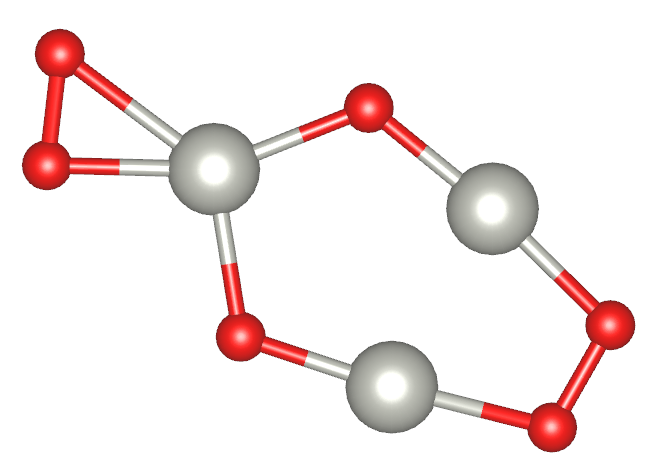
    Example of adsorbed structures:

    Representative set extraction

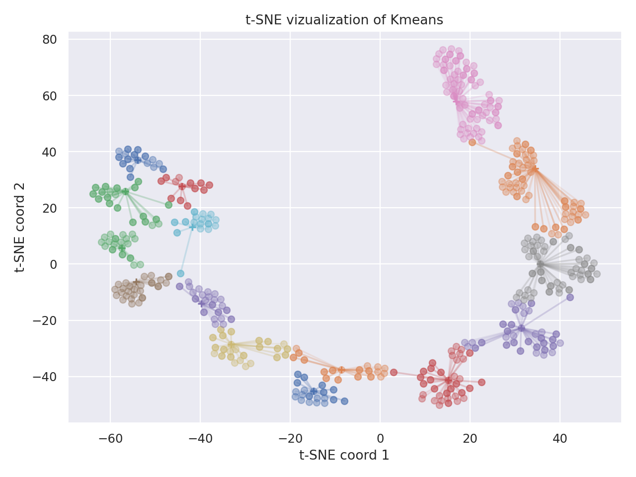
    Finaly, the structures in poll are clusterized with K-means yielding a representative set. The structures are written in folder_xyz_files (adsorbed structures) and folder_xyz_files_withsurfs (adsorbed structures with surface information). A vizualization of the clustering process is indicated in the file clustering_representatives*.png.

    The code

    Required packages

    • numpy
    • scipy
    • argparse
    • pandas
    • sklearn
    • matplotlib

    Running the code

    Example with required arguments:

    $ cd example
    $ python ../adsorption.py --mols            A.xyz B.xyz \\
                              --chem_envs       20 5        \\
                              --n_final         50

    Example with all arguments:

    $ cd example
    $ python ../adsorption.py --mols            A.xyz B.xyz \\
                              --chem_envs       20 5        \\
                              --n_final         50          \\
                              --n_rot           60          \\
                              --surf_d          10          \\
                              --n_repeat_km     20          \\
                              --ovlp_threshold  0.95        \\
                              --sim_threshold   0.04        \\
                              --out_sufix       _teste

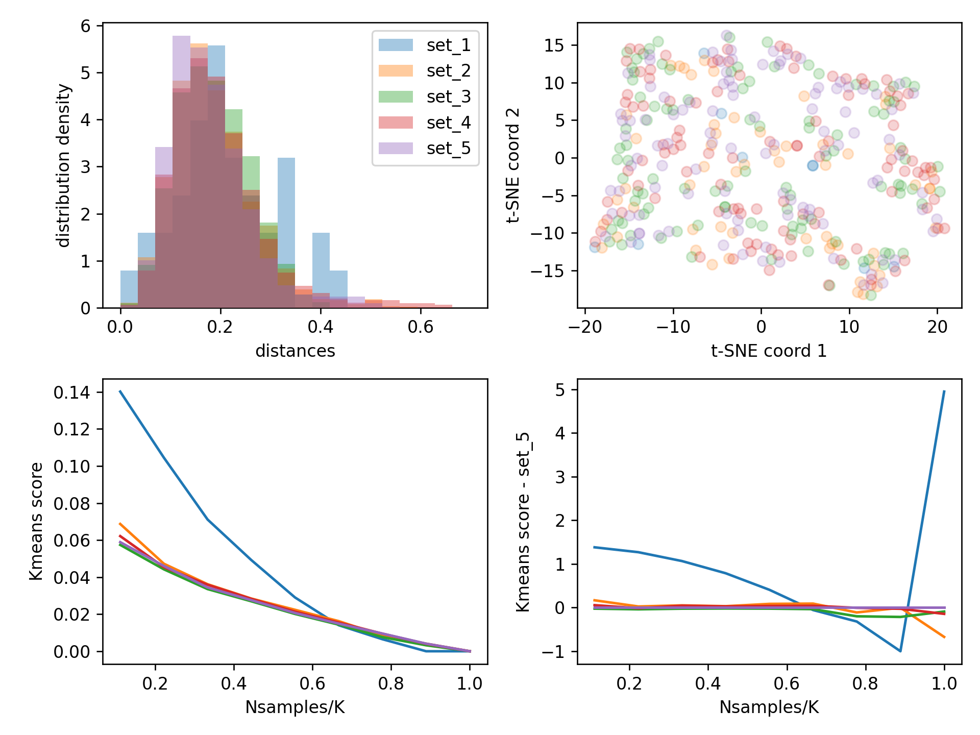
    Comparison of representative sets

    The script comparison.py allow to compare multiple sets of adsorbed molecules, for instance, generated with different parameters. It read the molecules in the xyz format, in saparated folders, and get features for they. The features are the same of the employed in the adsorption step described above, if the size of the adsorbed molecules presented in the order of the xyz file. Otherwise, it employs a single key point, the geometric center of the system, which should decrease the quality of the description of the features.

    Then, few analysis/plots are performed with this data:

    • A histogram of distances among the samples;
    • A t-SNE dimensionality reduction;
    • A sequence of K-means clustering, increasing K/data size de approximatated 0 a 1.

    The results are saved to a file named result_comparison.png:

    Running the code

    $ cd example
    $ python ../comparison.py --folders set_1 set_2 set_3 set_4 set_5 --subs_ns 9 3
    Visit original content creator repository https://github.com/johnatanmucelini/Molecular-Binding-Algorithm-by-Surface-Mapping-MBASM
  • deep-learning-challenge

    Module 21 Report – deep-learning-challenge.

    Overview.

    The purpose of this analysis was to use my knowledge of machine learning and neural networks to create a binary classifier that can predict whether applicants will be successful if funded by Alphabet Soup.
    The funding information of more than 34,000 organisations that have received funding from Alphabet Soup over the years was imported from the <charity_data.csv> and included (12 columns and 34298 rows, excluding the Header):

    • EIN
    • NAME
    • APPLICATION_TYPE
    • AFFILIATION
    • CLASSIFICATION
    • USE_CASE
    • ORGANIZATION
    • STATUS
    • INCOME_AMT
    • SPECIAL_CONSIDERATIONS
    • ASK_AMT
    • IS_SUCCESSFUL (0 label = unsuccessful, 1 label = successful)

    <AlpahabetSoupCharity.ipynb> for the original machine learning model.
    <AlpahabetSoupCharity_Optimisation_keras_tuner.ipynb> for use of an autotuner to find best model hyperparameters.
    <AlpahabetSoupCharity_Optimisation.ipynb> for the process described below.

    Results

    Data Preprocessing

    What variable(s) are the target(s) for your model?

    • The “IS_SUCCESSFUL” column, was the y target variable for the model.
    • There were 18261 1 successful labels and 16038 0 unsuccessful labels. This indicated a fairly well-balanced column of data as the target variable.

    What variable(s) are the features for your model?

    • All other columns, excluding “EIN”, are the X variable or features for the model.

    What variable(s) should be removed from the input data because they are neither targets nor features?

    • The “EIN” column was removed from the input data because it was an identification column ( each EIN was a unique value) and neither a target nor feature.

    • The “NAME” column is also an identification column, but I added this into the input data as the value-counts of this column (not all names were unique) indicated that many organisations had applied for funding on multiple occassions, hence the frequency of their application for funding may contribute to success in being funded.
    • The “NAME” column had any organisations that applied less than 206 times (value_counts) for funding, “binned” together in a new value called “Other”. So there were 15 unique values for this column.

    • The “CLASSIFICATION” column had 71 unique values, so any values with less than 58 value_counts, were “binned” together in a new value called “Other”. So there were 15 unique values for this column.

    • The “APPLICATION” column had 17 unique values, I kept all of these, no binning.

    • The “AFFILIATION” column had 6 unique values, I kept all of these, no binning.

    • The “INCOME_AMT” column had 9 unique values, I kept all of these, no binning.

    • The “USE_CASE” column had 5 unique values, I kept all of these, no binning.

    • The “ORGANISATION” column had 4 unique values, I kept all of these, no binning.

    • I used the OneHotEncoder to convert all categorical columns into numerical data, as an alternative method to using get_dummies. These columns were then merged with the numerical columns.

    • I then chose to drop the column ‘SPECIAL_CONSIDERATIONS_N’ as values for this were already contained in the ‘SPECIAL_CONSIDERATIONS_Y’ column.

    • The final DataFrame had 75 columns.

    • Data was split using “train_test_split”.

    • Data was then scaled as the “ASK_AMT” column was a much larger integer compared with all other columns.

    Compiling, Training, and Evaluating the Model

    How many neurons, layers, and activation functions did you select for your neural network model, and why?

    • The features for the model were 74 in total.

    • The length of X-train, 74, was the input-dimensions for the input layer, with 74 neurons. I experimented with relu, LeakyReLu and tanh activation functions, and got best results with a tanh activation function.

    • In the 2nd hidden layer I chose to use two thirds the input layer of neurons, selecting 50. I experimented with relu, LeakyReLu and tanh activation functions, and got best results with a tanh activation function.

    • In the output layer there was 1 neuron and a sigmoid activation function used.

    • There were 9351 parameters in this model.

    • I was also able to create a callback that saved the model weights every five epochs. These were saved in a checkpoint folder in content in colab.

    Were you able to achieve the target model performance?

    • I am so EXCITED to say I achieved the target model performance of 75% accuracy.

    What steps did you take in your attempts to increase model performance?

    • Experimenting with binning fewer features so as to have more columns in the Dataframe.
    • Increasing the number of neurons/nodes in each hidden layer.
    • I experimented with a 3rd hidden layer, but this did not improve accuracy or reduce loss.
    • I tried an optimisation with adamW and a learning-rate.
    • I also experimented with a dropout activation in alayer.
    • I used relu, tanh and leakyrelu activation fucntion in each, all or alternating layers.
    • I also experimented with increasing epochs.
    • Changing the train_test_split with train-size = 0.2, rather than the deafult setting of 0.25, was also tried, but this did not help the model convergence.

    Summary.

    The deep learning model optimisation <AlpahabetSoupCharity_Optimisation.ipynb> achieved an improved accuracy and reduced loss when compared with the first model <AlpahabetSoupCharity.ipynb>.

    First model
    Loss: 0.5581400394439697, Accuracy: 0.7292128205299377

    Optimisation model
    Loss: 0.5132946372032166, Accuracy: 0.7500874400138855

    I also ran a keras tuner to find the best 3 model hyperparameters, <AlpahabetSoupCharity_Optimisation_keras_tuner.ipynb>.

    I would recommend the use of a logistic regression model, a support vector machine learning model or a decision tree to improve prediction accuracy with this classification problem of what features contribute to improved success in getting funding from the Alphabet Soup organisation.

    Enjoy marking! Sandra

    Visit original content creator repository
    https://github.com/SandraBotica/deep-learning-challenge

  • pokeMONS-EE298

    pokeMONS-EE298

    Machine Problem Submissions for EE298

    pip install -r requirements.txt

    Machine Problem 1: Hashing v16

    Implementing SHA-512 Hashing Algorithm in Python

    • accepts both file and string input
    python3 sha512.py "hello world"
    python3 sha512.py input.pdf
    • accepts benchmarking tests using hashlib module in sota_sha512.py
    python3 benchmark_sha512.py "hello world!"
    • to download 100MB test file, you may use the sample below
    curl -O https://files.testfile.org/PDF/10MB-TESTFILE.ORG.pdf
    curl -O https://files.testfile.org/PDF/100MB-TESTFILE.ORG.pdf

    Machine Problem 2: Port Scanner v16

    Implementing an NMAP-like Port Scanner in Python

    • uses NMAP-like syntax to accept hostnames, individual and ranges of ip addresses, and even a subnet in CIDR notation
    python3 port_scanner.py scanme.nmap.org
    python3 port_scanner.py 202.92.128.1
    python3 port_scanner.py 202.92.127-128.1-204
    python3 port_scanner.py 202.92.1/24
    • uses NMAP-like syntax to accept individual and ranges of ports using -p tag
    python3 port_scanner.py 202.92.128.1 -p 22,30-50,80,100-1000
    • use -O tag to enable OS Detection *requires root access
    • use -sV tag to enable Service Info Detection
    sudo python3 port_scanner.py scanme.nmap.org -sV -O
    • use -sU tag to opt for UDP Scanning of port 53 and 161 *disables OS detection and Service Info Detection
    python3 port_scanner.py scanme.nmap.org -sU

    Visit original content creator repository
    https://github.com/reddiedev/pokeMONS-EE298

  • Beers-Statistical-Analysis-R

    Data Dictionary

    Variable Description
    Name The name of the beer
    Style The style of the beer
    Brewery The name of the brewery of the beer
    ABV The ABV (Alcohol by Volume) of the beer
    rating The rating of the beer in a scale of 1-5
    minIBU The minimum IBU (International Bitterness Units scale) score of the beer
    maxIBU The maximum IBU (International Bitterness Units scale) score of the beer
    Astringency The Astringency score of the beer
    Body Describes how heavy or light the beer is
    Alcohol The alcohol content in the beer
    Bitter The score of the beer having bitter elements in its flavour
    Sweet The score of the beer having sweet elements in its flavour
    Sour The score of the beer having sour elements in its flavour
    Salty The score of the beer having salty elements in its flavour
    Fruits The score of the beer having fruity elements in its flavour
    Hoppy The score of the beer having hoppy elements in its flavour
    Spices The score of the beer having spicy elements in its flavour
    Malty The score of the beer having malty elements in its flavour


    Visit original content creator repository
    https://github.com/ecemuzun/Beers-Statistical-Analysis-R